`harmonic_ud_grade` vs `ud_grade`: A Focused Comparison#

When working with HEALPix maps, it is often necessary to change the resolution — for example, to downgrade a high-resolution observation map to a lower Nside for comparison with a model, or to reduce computational cost for large-scale analyses.

healpy provides two functions for this:

ud_grade: operates purely in pixel space by averaging groups of sub-pixels. It is fast, but because it does not apply any anti-aliasing filter, high-multipole power from the input grid “folds” back into the output — a phenomenon known as aliasing.
harmonic_ud_grade: operates in spherical-harmonic space. It decomposes the input map into \(a_{\ell m}\) coefficients, can apply the pixel-window correction following the prescription in Planck Collaboration 2015 X, and optionally scales the beam. Because the harmonic transform band-limits the output, high-ell aliasing is strongly suppressed.

How `harmonic_ud_grade` works#

The function implements the following per-\(\ell\) transfer (Planck Collaboration 2015 X):

\[a^{\rm out}_{\ell m} = \frac{p^{\rm out}_\ell}{p^{\rm in}_\ell} \cdot \frac{b^{\rm out}_\ell}{b^{\rm in}_\ell} \cdot a^{\rm in}_{\ell m}\]

where \(p_\ell\) is the HEALPix pixel-window function and \(b_\ell\) is a Gaussian beam transfer function. The pixel-window ratio is included when pixwin=True; otherwise that factor is omitted. The algorithm proceeds in three steps:

Analysis: The input map is decomposed into \(a_{\ell m}\) via map2alm (using pixel weights by default for high accuracy).
Transfer: Each \(a_{\ell m}\) is multiplied by the requested output/input pixel-window and beam ratios. Modes above \(\ell_{\max}^{\rm out}\) are discarded (band-limiting).
Synthesis: The modified \(a_{\ell m}\) are synthesized into a map at nside_out via alm2map.

Quick Guide#

Use the method that matches the map content and science target:

Input / Goal	Prefer	Why
Diffuse sky maps, CMB-like fields, power spectra	`harmonic_ud_grade`	Band-limits before synthesis and can handle pixel-window/beam transfer.
Beam-convolved diffuse maps	`harmonic_ud_grade` with the correct `fwhm_in`; consider `fwhm_out=None`	Preserves spectral content while controlling the output effective beam.
Binary masks, hit-count maps, catalog/source templates	`ud_grade`	These are pixel-localized quantities; harmonic truncation can ring.
Mixed diffuse + compact emission	Separate components when possible	Downgrade diffuse emission harmonically and compact/mask-like components in pixel space.

The examples below use use_pixel_weights=False so the notebook runs quickly and without downloading HEALPix pixel-weight files. For production analysis, keep the default use_pixel_weights=True when accuracy is more important than runtime.

[1]:

import time
import numpy as np
import healpy as hp
import matplotlib.pyplot as plt

plt.rcParams.update({"figure.dpi": 120, "font.size": 11})

# Note: the examples below pass `use_pixel_weights=False` so the notebook
# runs without downloading the HEALPix pixel-weight files.  In production
# code keep the default `use_pixel_weights=True` for the most accurate SHT.

print(f"healpy {hp.__version__}")
print(f"Effective resolution beam at NSIDE 64: {hp.effective_resolution_fwhm(64, arcmin=True):.1f} arcmin")

healpy 1.20.0b2.dev23+gad776d288
Effective resolution beam at NSIDE 64: 160.0 arcmin

[2]:

def paint_gaussian_sources(nside, source_pixels, sigma, amplitudes):
    """Paint Gaussian source profiles centered on HEALPix pixels."""
    source_vecs = np.array(hp.pix2vec(nside, source_pixels)).T
    all_vecs = np.array(hp.pix2vec(nside, np.arange(hp.nside2npix(nside)))).T

    output = np.zeros((len(amplitudes), hp.nside2npix(nside)))
    for source_vec in source_vecs:
        cos_dist = np.clip(np.dot(all_vecs, source_vec), -1, 1)
        ang_dist = np.arccos(cos_dist)
        profile = np.exp(-0.5 * (ang_dist / sigma) ** 2)
        for i, amplitude in enumerate(amplitudes):
            output[i] += amplitude * profile

    return output[0] if len(amplitudes) == 1 else output

1. Aliasing Stress Test: A Single High-\(\ell\) Mode#

The simplest way to reveal aliasing is to construct a pathological input: a map at nside_in = 128 that contains power at exactly one spherical-harmonic multipole, \(\ell = 120\).

The target resolution is nside_out = 32, whose maximum resolvable multipole is \(\ell_{\max} = 3 \times 32 - 1 = 95\). Since \(\ell = 120 > \ell_{\max}\), a correct downgrade must produce an output whose target-band power is suppressed to the numerical SHT residual level.

Key parameter choices:

pixwin=True is passed both when creating the input map (alm2map) and when calling harmonic_ud_grade. This simulates a realistic pixelized observation and allows harmonic_ud_grade to properly deconvolve the input pixel window and apply the output pixel window.
fwhm_in=0 because the synthetic input has no instrumental beam.

[3]:

nside_in = 128
nside_out = 32
lmax_out = 3 * nside_out - 1

# Single mode at ell=120
alm_single = np.zeros(hp.Alm.getsize(120), dtype=np.complex128)
alm_single[hp.Alm.getidx(120, 120, 0)] = 1.0
# Generate the synthetic map with pixwin=True so it has a realistic pixel
# window; harmonic_ud_grade will deconvolve it as part of the transfer.
m_in = hp.alm2map(alm_single, nside=nside_in, pixwin=True)

# Downgrade methods
m_ud = hp.ud_grade(m_in, nside_out=nside_out)

# fwhm_in=0 because the synthetic input has no instrumental beam
m_harm = hp.harmonic_ud_grade(
    m_in,
    nside_out=nside_out,
    fwhm_in=0,
    use_pixel_weights=False,
    pixwin=True,
    fwhm_out=0,
)

cl_in = hp.anafast(m_in)
cl_ud = hp.anafast(m_ud)
cl_harm = hp.anafast(m_harm)

plt.figure(figsize=(10, 5))
plt.semilogy(np.maximum(cl_in, 1e-8), label=f"Input (Nside={nside_in})", color="black", linestyle="--")
plt.semilogy(np.maximum(cl_ud, 1e-8), label=f"ud_grade (Nside={nside_out})", alpha=0.8)
plt.semilogy(np.maximum(cl_harm, 1e-8), label=f"harmonic_ud_grade (Nside={nside_out})", alpha=0.8)
plt.axvline(lmax_out, color="red", ls=":", label=r"Output $\ell_{\max}$")
plt.xlabel(r"$\ell$")
plt.ylabel(r"$C_\ell$")
plt.xlim(0, 150)
plt.ylim(1e-8, cl_in.max() * 5)
plt.title("Aliasing of a single high-frequency mode ($\\ell=120$)")
plt.legend()
plt.grid(alpha=0.3)
plt.tight_layout()
plt.show()

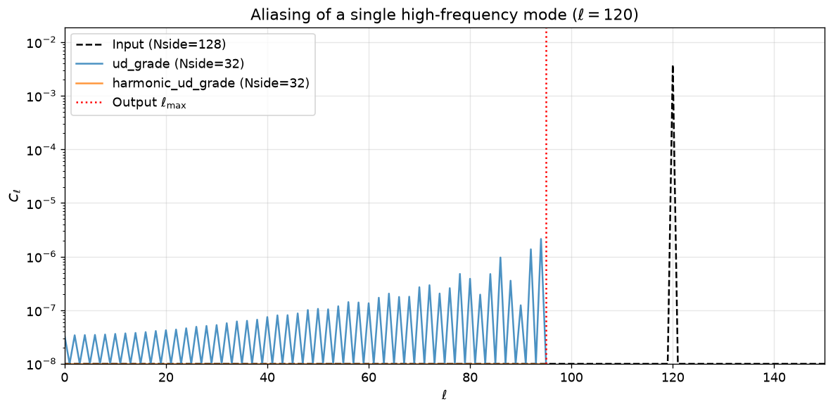
_images/healpy_harmonic_ud_grade_comparison_5_0.png

Interpretation of the plot above:

Black dashed line (Input): The input power spectrum has a sharp peak at \(\ell = 120\) and is essentially zero everywhere else. The satellite peaks visible near \(\ell = 120\) come from the finite pixelization of the nside_in = 128 grid: a single harmonic mode painted onto a discrete pixel grid is no longer perfectly monochromatic, so a small amount of power leaks into nearby multipoles.
Blue line — ``ud_grade``: Significant spurious power appears across the entire output multipole range. This is aliasing: because pixel-space averaging has no frequency cutoff, the high-\(\ell\) mode is “folded” back into the lower multipoles, corrupting the output with an oscillating pattern.
Orange line — ``harmonic_ud_grade``: The output spectrum is near the numerical floor across the output multipole range — the expected result for this synthetic setup. The harmonic transform naturally band-limits the result to \(\ell \le \ell_{\max}\), so the \(\ell = 120\) mode is cleanly removed.
Red dotted line: The output bandlimit \(\ell_{\max} = 95\).

The RMS values printed below make this quantitative: ud_grade retains a large fraction of the original map RMS as pure aliasing artifact, while harmonic_ud_grade suppresses it to the numerical noise floor.

[4]:

print(f"Input map RMS:              {np.std(m_in):.6e}")
print(f"ud_grade output RMS:        {np.std(m_ud):.6e}  <-- aliasing")
print(f"harmonic_ud_grade RMS:      {np.std(m_harm):.6e}  <-- suppressed")

Input map RMS:              2.705287e-01
ud_grade output RMS:        1.154352e-01  <-- aliasing
harmonic_ud_grade RMS:      6.952337e-04  <-- suppressed

2. Power-Spectrum Recovery — Why It Matters#

The single-mode test above is deliberately extreme. Real sky maps contain power at all multipoles, so aliasing from ud_grade is spread across the full spectrum, making it harder to spot by eye but no less damaging to science.

In this section we synthesize a realistic broadband signal with \(C_\ell \propto \ell^{-2}\) (a spectrum often used for test purposes) at nside_in = 256, downgrade to nside_out = 64, and compare the recovered power spectrum against a ground-truth reference.

The reference is built by truncating the original \(a_{\ell m}\) to \(\ell_{\max}^{\rm out}\) and synthesizing directly at the output resolution, so both the reference and the downgraded maps contain the same pixel-window effects. Any difference between them is therefore purely due to the downgrade method.

[5]:

nside_in = 256
nside_out = 64
lmax_in = 3 * nside_in - 1
lmax_out = 3 * nside_out - 1

np.random.seed(42)  # synalm draws random alm from the global RNG
ell = np.arange(lmax_in + 1, dtype=float)
cl_in = np.zeros(lmax_in + 1)
cl_in[2:] = ell[2:] ** (-2.0)
elm = hp.synalm(cl_in, lmax=lmax_in)
m_in = hp.alm2map(elm, nside=nside_in, lmax=lmax_in, pixwin=True)

# Ground-truth reference: directly synthesize at output resolution
elm_ref = hp.resize_alm(elm, lmax_in, lmax_in, lmax_out, lmax_out)
m_ref = hp.alm2map(elm_ref, nside=nside_out, lmax=lmax_out, pixwin=True)

m_ud = hp.ud_grade(m_in, nside_out=nside_out)

# fwhm_in=0 for this synthetic simulation with no beam
m_harm = hp.harmonic_ud_grade(
    m_in,
    nside_out=nside_out,
    fwhm_in=0,
    use_pixel_weights=False,
    pixwin=True,
    fwhm_out=0,
)

# Measure spectra
cl_ref = hp.anafast(m_ref, lmax=lmax_out)
cl_ud = hp.anafast(m_ud, lmax=lmax_out)
cl_harm = hp.anafast(m_harm, lmax=lmax_out)
ell_out = np.arange(lmax_out + 1)

[6]:

fig, axes = plt.subplots(1, 2, figsize=(12, 4))

axes[0].loglog(ell_out[2:], cl_ref[2:], "k--", lw=2, label="Reference $C_\ell$ (truth)")
axes[0].loglog(ell_out[2:], cl_ud[2:], alpha=0.8, label="ud_grade")
axes[0].loglog(ell_out[2:], cl_harm[2:], alpha=0.8, label="harmonic_ud_grade")
axes[0].axvline(lmax_out, color="red", ls=":", label=r"$\ell_{\max}$")
axes[0].set_xlabel(r"$\ell$")
axes[0].set_ylabel(r"$C_\ell$")
axes[0].set_title("Power spectra after downgrade")
axes[0].legend()
axes[0].grid(alpha=0.3)

# Fractional error
frac_ud = (cl_ud[2:] - cl_ref[2:]) / cl_ref[2:]
frac_harm = (cl_harm[2:] - cl_ref[2:]) / cl_ref[2:]

axes[1].plot(ell_out[2:], frac_ud * 100, alpha=0.8, label="ud_grade")
axes[1].plot(ell_out[2:], frac_harm * 100, alpha=0.8, label="harmonic_ud_grade")
axes[1].axhline(0, color="k", lw=0.5)
axes[1].axvline(lmax_out, color="red", ls=":")
axes[1].set_xlabel(r"$\ell$")
axes[1].set_ylabel("Fractional error [%]")
axes[1].set_title("Spectral error vs truth")
axes[1].legend()
axes[1].grid(alpha=0.3)

plt.tight_layout()
plt.show()

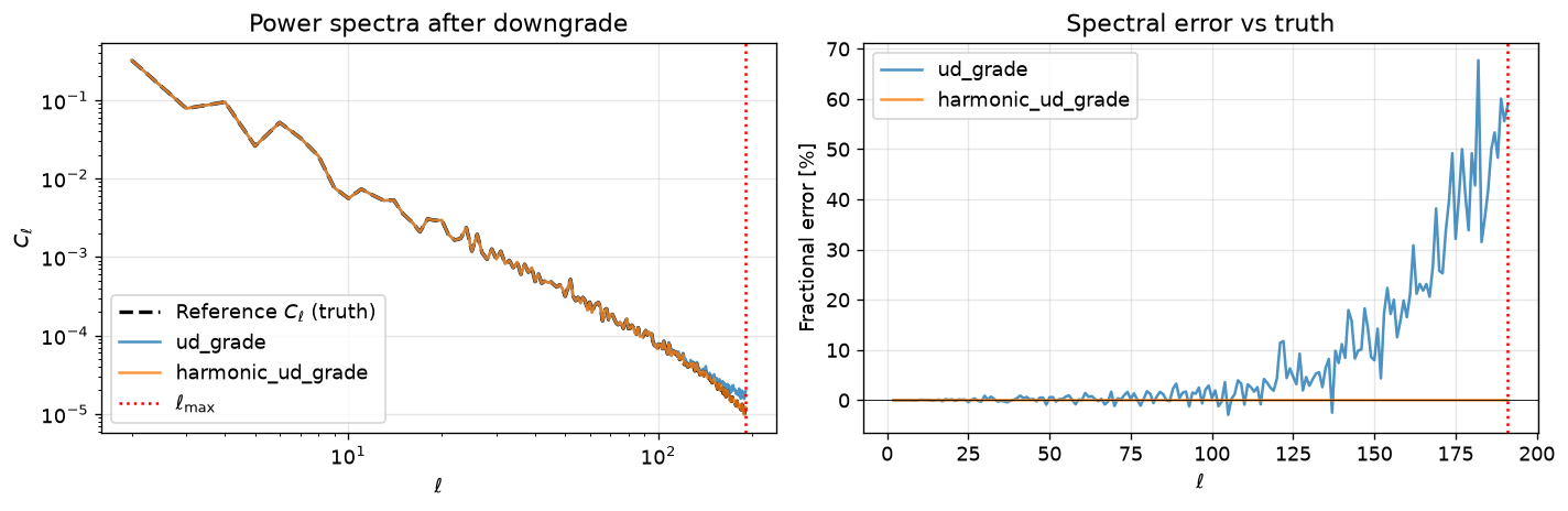
_images/healpy_harmonic_ud_grade_comparison_10_0.png

Interpretation of the plots above:

Left panel — Power spectra after downgrade: All three curves agree well at low \(\ell\), but diverge at high multipoles. The reference (black dashed) and harmonic_ud_grade (orange) both roll off smoothly beyond \(\ell \approx 100\): this is the expected damping from the pixel window of the nside_out = 64 grid. ud_grade (blue), by contrast, shows a visible excess of power in this regime because aliased high-frequency structures from above \(\ell_{\max}\) have been folded back into the output.

Right panel — Fractional spectral error relative to truth: This panel makes the aliasing bias quantitative.

harmonic_ud_grade (orange) sits flat on 0 % error — it tracks the truth map closely for this band-limited synthetic signal.
ud_grade (blue) is systematically positive, meaning it over-estimates the power. This is the behavior of this broadband example: aliased high-ell variance appears as a positive high-ell bias. The error grows rapidly toward \(\ell_{\max}\), reaching 50–70 % near the bandlimit.

Because both the reference and the downgraded maps include the same pixel window, window effects largely cancel in the ratio. The remaining difference is dominated by downgrade artifacts and SHT residuals.

The RMS fractional error below summarizes this over the “safe” multipole band \(\ell \in [2,\, 2 N_{\rm side}^{\rm out}]\):

[7]:

safe = slice(2, 2 * nside_out + 1)
print(
    f"RMS frac. error over safe band ℓ ∈ [2, {2*nside_out}]:\n"
    f"  ud_grade:          {np.sqrt(np.mean(frac_ud[safe]**2))*100:.2f}%\n"
    f"  harmonic_ud_grade: {np.sqrt(np.mean(frac_harm[safe]**2))*100:.2f}%"
)

RMS frac. error over safe band ℓ ∈ [2, 128]:
  ud_grade:          2.34%
  harmonic_ud_grade: 0.00%

Expected aliasing from the input spectrum#

The ud_grade excess is not mysterious — it is predicted by the input power spectrum. ud_grade performs pixel averaging without bandlimiting, so modes above \(\ell_{\max}^{\rm out}\) alias into the output. For a power-law spectrum \(C_\ell \propto \ell^{-2}\), roughly 27 % of the total power sits above the output bandlimit and folds back.

We can estimate the aliased power fraction analytically:

[8]:

# Estimate the fraction of input power above the output bandlimit
# that ud_grade aliases into the output
ell_full = np.arange(lmax_in + 1, dtype=float)
power_below = np.sum(cl_in[2:lmax_out+1] * (2*ell_full[2:lmax_out+1] + 1))
power_above = np.sum(cl_in[lmax_out+1:] * (2*ell_full[lmax_out+1:] + 1))
alias_frac = power_above / (power_below + power_above)

print(f"Input spectrum: C_ell ~ ell^(-2)")
print(f"  Power below ell_max={lmax_out}: {power_below:.2f}")
print(f"  Power above ell_max={lmax_out}: {power_above:.2f}")
print(f"  Aliasing fraction: {alias_frac*100:.1f}%")
print()
print("Compare with observed ud_grade excess at high ell:")
high_ell = slice(lmax_out - 20, lmax_out + 1)
observed_excess = np.mean(cl_ud[high_ell]) / np.mean(cl_ref[high_ell]) - 1
print(f"  Mean excess at ell ~ {lmax_out-10}-{lmax_out}: {observed_excess*100:.0f}%")
print(f"  (Aliasing concentrates near the bandlimit, so the per-bin")
print(f"   excess at high ell exceeds the total power fraction.)")

Input spectrum: C_ell ~ ell^(-2)
  Power below ell_max=191: 10.30
  Power above ell_max=191: 2.78
  Aliasing fraction: 21.2%

Compare with observed ud_grade excess at high ell:
  Mean excess at ell ~ 181-191: 44%
  (Aliasing concentrates near the bandlimit, so the per-bin
   excess at high ell exceeds the total power fraction.)

3. Noise Aliasing — The Real-World Failure Mode#

The tests above used noiseless inputs, but real observational data always contain instrumental noise. In CMB data processing a particularly important case is blue noise — noise whose power spectrum grows with \(\ell\) (e.g., \(C_\ell^{\rm noise} \propto \ell^{2}\)). This commonly arises when a map is beam-deconvolved: dividing out the beam’s Gaussian roll-off amplifies the high-frequency noise enormously.

Because ud_grade operates in pixel space with no frequency cutoff, that amplified high-\(\ell\) noise above \(\ell_{\max}^{\rm out}\) can leak back into the signal band, dramatically raising the noise floor. harmonic_ud_grade avoids this by band-limiting the map before downgrading.

Below we construct a signal + blue-noise map at nside_in = 256, downgrade to nside_out = 64 (a factor-4 step), and isolate the noise contribution in each output. The resolution step still leaves high-\(\ell\) noise power above \(\ell_{\max}^{\rm out} = 191\) that can alias back.

[9]:

nside_in = 256
nside_out = 64
lmax_out = 3 * nside_out - 1

np.random.seed(42)  # synfast draws random alm from the global RNG
ell_in = np.arange(3 * nside_in + 1, dtype=float)
cl_signal = np.zeros(3 * nside_in + 1)
cl_signal[2:] = ell_in[2:] ** (-2.0)
map_signal = hp.synfast(cl_signal, nside_in, lmax=3 * nside_in, new=True, pixwin=True)

# Blue noise: noise dominates at high ℓ (e.g. beam deconvolved noise)
ell_knee = 50
cl_noise = np.zeros(3 * nside_in + 1)
cl_noise[2:] = cl_signal[ell_knee] * (ell_in[2:] / ell_knee) ** 2
# pixwin=False: noise is a pixel-level quantity, not a smooth sky signal.
# Applying the pixel window to noise would incorrectly suppress its
# high-ell power, understating the aliasing problem.
map_noise = hp.synfast(cl_noise, nside_in, lmax=3 * nside_in, new=True, pixwin=False)
map_noisy = map_signal + map_noise

# Reference: downgrade signal-only with harmonic
m_ref_signal = hp.harmonic_ud_grade(
    map_signal,
    nside_out=nside_out,
    fwhm_in=0,
    use_pixel_weights=False,
    pixwin=True,
    fwhm_out=0,
)

# Downgrade methods
m_ud = hp.ud_grade(map_noisy, nside_out=nside_out)
m_harm = hp.harmonic_ud_grade(
    map_noisy,
    nside_out=nside_out,
    fwhm_in=0,
    use_pixel_weights=False,
    pixwin=True,
    fwhm_out=0,
)

# Isolate noise contribution
cl_noise_ud = hp.anafast(m_ud - hp.ud_grade(map_signal, nside_out=nside_out), lmax=lmax_out)
cl_noise_harm = hp.anafast(m_harm - m_ref_signal, lmax=lmax_out)
cl_signal_out = hp.anafast(m_ref_signal, lmax=lmax_out)

[10]:

plt.figure(figsize=(8, 5))

plt.loglog(ell_out[2:], cl_signal_out[2:], "k--", lw=2, label="Signal (truth)")
plt.loglog(ell_out[2:], cl_noise[:lmax_out + 1][2:], "gray", ls=":", lw=2, label="Input Noise")
plt.loglog(ell_out[2:], cl_noise_ud[2:], alpha=0.8, label="Noise in ud_grade")
plt.loglog(ell_out[2:], cl_noise_harm[2:], alpha=0.8, label="Noise in harmonic_ud_grade")
plt.xlabel(r"$\ell$")
plt.ylabel(r"$C_\ell$ (noise)")
plt.title("Noise contamination after downgrade")
plt.legend()
plt.grid(alpha=0.3)
plt.tight_layout()
plt.show()

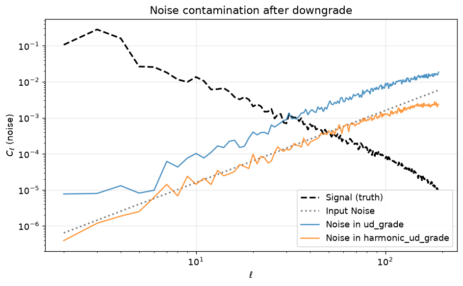
_images/healpy_harmonic_ud_grade_comparison_17_0.png

Interpretation of the plot above:

This plot isolates the noise-only component after downgrading from nside = 256 to nside = 64 (a factor-8 resolution step). Each curve has a specific meaning:

Black dashed (Signal truth): The true signal power spectrum at the output resolution. It is shown for context so you can judge where noise starts to dominate over signal.
Grey dotted (Input Noise): The raw analytic noise spectrum \(C_\ell^{\rm noise} \propto \ell^{2}\) as injected into the input map. It crosses the signal near \(\ell \approx 50\) (the chosen knee multipole) and grows steeply beyond.
Orange: harmonic_ud_grade The noise residual after harmonic downgrading. It tracks the input noise closely at low \(\ell\) and rolls off above \(\ell \approx 100\) due to the target pixel window — exactly as expected.
Blue: ud_grade The noise residual after pixel-space downgrading. Across the full multipole range, the ud_grade noise is roughly higher than the harmonic_ud_grade noise. This excess is entirely due to aliased high-\(\ell\) noise being folded into the signal band. The effect grows with the resolution ratio: a larger step means more high-\(\ell\) modes available to alias, producing a larger noise floor uplift.

Notes on the noise model:

Noise is generated with pixwin=False because instrumental noise is a pixel-level quantity — it does not have a smooth pixel window like sky emission. Using pixwin=True for noise would incorrectly suppress its high-\(\ell\) power and understate the aliasing problem.
The \(C_\ell \propto \ell^{2}\) spectrum is a proxy for beam-deconvolved noise, but is not exactly equivalent: a truly deconvolved noise map would have its power amplified by \(1/b_\ell^{2}\), which diverges at high \(\ell\). For a precise simulation, generate white noise and then explicitly deconvolve the beam. The \(\ell^{2}\) proxy is sufficient here to demonstrate the aliasing effect.
For white noise (\(C_\ell = \mathrm{const}\)), ud_grade works well because the pixel-averaging naturally reduces the noise variance by the ratio of pixel areas. The aliasing advantage of harmonic_ud_grade is specific to noise with rising high-\(\ell\) power spectra.

Why this matters in practice: When analyzing real CMB or astrophysical data, any aliased noise that leaks into the low-\(\ell\) modes will bias power-spectrum estimates, cross-correlations, and component-separation results. harmonic_ud_grade mitigates this by applying a harmonic bandlimit before re-gridding to the output resolution.

4. When `ud_grade` Wins: Point Sources and Gibbs Ringing#

The previous sections show why harmonic_ud_grade is often better for broadband or high-ell-noisy diffuse signals. But there is an important case where ud_grade is the better choice: maps dominated by compact, localized features such as point sources or binary masks.

A point source is a delta function on the sky, which means it has power at all multipoles. When harmonic_ud_grade band-limits the map to \(\ell_{\max}^{\rm out}\), it truncates the harmonic expansion abruptly, producing oscillating Gibbs ringing around each source. ud_grade, operating purely in pixel space, simply averages the sub-pixels and preserves the compact, positive-definite nature of the source.

To make this test realistic, we simulate point sources as an instrument would observe them: we paint a Gaussian beam profile directly in pixel space at each source position, using the Planck-suggested FWHM for the input resolution. We then compare three downgrade strategies:

ud_grade — pixel-space averaging.
harmonic_ud_grade with fwhm_out = 0 — band-limit only, no additional smoothing.
harmonic_ud_grade with fwhm_out=None — effective resolution beam (Planck-scaled output beam).

[11]:

nside_in = 256
nside_out = 64

# Effective resolution beam at this NSIDE
fwhm_in_pts = hp.effective_resolution_fwhm(nside_in)
sigma_in = fwhm_in_pts / (2 * np.sqrt(2 * np.log(2)))
print(f"Nside_in = {nside_in}, fwhm_in = {hp.effective_resolution_fwhm(nside_in, arcmin=True):.1f} arcmin "
      f"(effective resolution beam)")

# Simulate point sources as an instrument would see them:
# paint Gaussian beam profiles directly in pixel space.
rng = np.random.default_rng(123)
src_pixels = rng.choice(hp.nside2npix(nside_in), size=5, replace=False)
m_pts = paint_gaussian_sources(nside_in, src_pixels, sigma_in, [100.0])

# Downgrade: three methods
m_pts_ud = hp.ud_grade(m_pts, nside_out=nside_out)

# harmonic_ud_grade with NO additional smoothing (band-limit only)
m_pts_harm_nosmooth = hp.harmonic_ud_grade(
    m_pts,
    nside_out=nside_out,
    fwhm_in=fwhm_in_pts,
    use_pixel_weights=False,
    pixwin=True,
    fwhm_out=0,
)

# harmonic_ud_grade with effective resolution beam (fwhm_out=None)
m_pts_harm_smooth = hp.harmonic_ud_grade(
    m_pts,
    nside_out=nside_out,
    fwhm_in=fwhm_in_pts,
    use_pixel_weights=False,
    pixwin=True,
    fwhm_out=None,
)

print(f"ud_grade:            min={m_pts_ud.min():.4f}, max={m_pts_ud.max():.2f}, "
      f"negative pixels: {(m_pts_ud < 0).sum()}")
print(f"harmonic (no smooth): min={m_pts_harm_nosmooth.min():.4f}, "
      f"max={m_pts_harm_nosmooth.max():.2f}, "
      f"negative pixels: {(m_pts_harm_nosmooth < 0).sum()}")
print(f"harmonic (eff. beam): min={m_pts_harm_smooth.min():.4f}, "
      f"max={m_pts_harm_smooth.max():.2f}, "
      f"negative pixels: {(m_pts_harm_smooth < 0).sum()}")

Nside_in = 256, fwhm_in = 40.0 arcmin (effective resolution beam)
ud_grade:            min=0.0000, max=34.85, negative pixels: 0
harmonic (no smooth): min=-3.9192, max=34.09, negative pixels: 24573
harmonic (eff. beam): min=-0.0003, max=5.79, negative pixels: 24369

[12]:

# Zoom in on one source with gnomview
theta, phi = hp.pix2ang(nside_in, src_pixels[0])
rot = (np.degrees(phi), 90 - np.degrees(theta))

fig = plt.figure(figsize=(16, 4))

ax1 = fig.add_subplot(141)
hp.gnomview(m_pts, rot=rot, reso=5, xsize=200,
            title=f"Input (Nside={nside_in})", hold=True, notext=True)

ax2 = fig.add_subplot(142)
hp.gnomview(m_pts_ud, rot=rot, reso=5, xsize=200,
            title=f"ud_grade (Nside={nside_out})", hold=True, notext=True)

ax3 = fig.add_subplot(143)
hp.gnomview(m_pts_harm_nosmooth, rot=rot, reso=5, xsize=200,
            title="harmonic (no smooth)", hold=True, notext=True)

ax4 = fig.add_subplot(144)
hp.gnomview(m_pts_harm_smooth, rot=rot, reso=5, xsize=200,
            title="harmonic (eff. beam)", hold=True, notext=True)

plt.show()

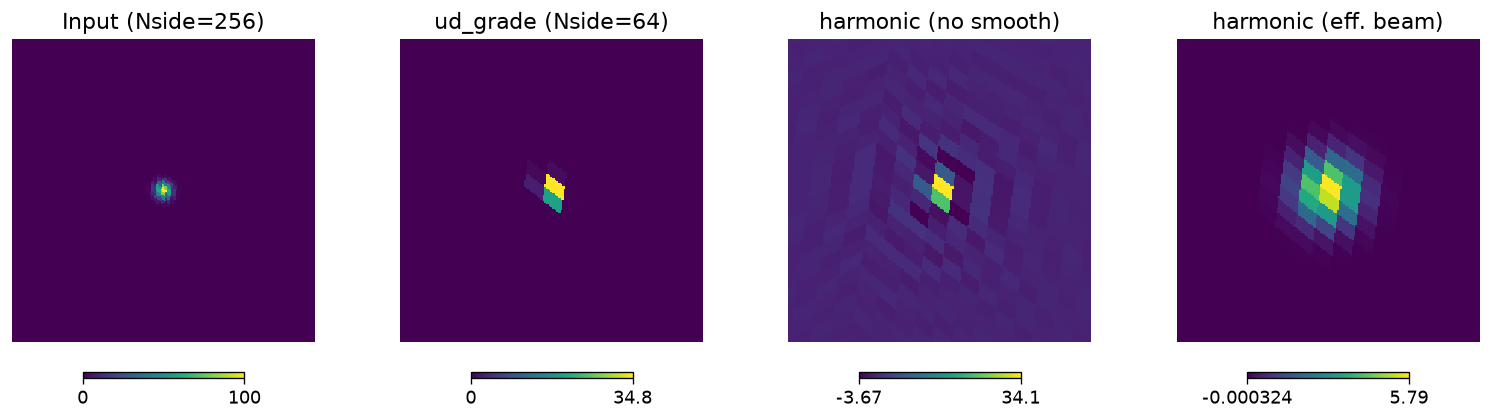
_images/healpy_harmonic_ud_grade_comparison_21_0.png

Interpretation of the plots above:

The four panels zoom in on one point source that was simulated with a realistic Gaussian beam painted directly in pixel space (FWHM ≈ 40 arcmin for Nside = 256).

Panel 1 (Input): The beam-convolved point source at the input resolution — a smooth Gaussian profile, as an instrument would observe it.
Panel 2: ud_grade Pixel-space averaging preserves the smooth, positive-definite profile of the beam. No ringing, no negative pixels.
Panel 3: harmonic_ud_grade (no smoothing) Band-limiting to \(\ell_{\max} = 191\) without additional smoothing produces visible Gibbs ringing — oscillations with negative values around the source. Even though the input is beam-convolved (not a true delta), the beam is narrow enough that significant power remains above \(\ell_{\max}^{\rm out}\), and truncating it causes ringing.
Panel 4: harmonic_ud_grade (effective resolution beam, fwhm_out=None) Applying the Planck-scaled effective resolution beam adds enough extra smoothing to suppress the ringing. This is the recommended harmonic approach for diffuse science — but for point-source work, ud_grade still produces a cleaner, more compact result.

Takeaway: harmonic_ud_grade is a good default for band-limited diffuse signals (CMB, diffuse emission). ud_grade is preferable for pixel-localized features (point sources, binary masks, hit-count maps).

4.1 Polarization (Q/U) with Point Sources#

The Gibbs-ringing problem is not limited to temperature maps. For polarization maps (TQU) containing compact features, the same band-limiting that harms point sources in \(T\) also produces ringing in \(Q\) and \(U\). This is particularly relevant for maps that contain both diffuse polarized emission (where harmonic_ud_grade excels) and localized polarized sources (where ud_grade is better).

Below we create a TQU map with point sources in all three components and compare the two methods.

[13]:

nside_in = 128
nside_out = 32

fwhm_in_pts = hp.effective_resolution_fwhm(nside_in)
sigma_in = fwhm_in_pts / (2 * np.sqrt(2 * np.log(2)))

# Create TQU maps with point sources
rng = np.random.default_rng(456)
src_pixels = rng.choice(hp.nside2npix(nside_in), size=3, replace=False)
m_pts_tqu = paint_gaussian_sources(nside_in, src_pixels, sigma_in, [100.0, 50.0, 30.0])

m_tqu_ud = hp.ud_grade(m_pts_tqu, nside_out=nside_out)
m_tqu_harm = hp.harmonic_ud_grade(
    m_pts_tqu, nside_out=nside_out, pol=True,
    fwhm_in=fwhm_in_pts, use_pixel_weights=False,
    pixwin=True, fwhm_out=0,
)

print("Point sources in TQU:")
print(f"  ud_grade Q  — negative pixels: {(m_tqu_ud[1] < 0).sum()}")
print(f"  harmonic Q  — negative pixels: {(m_tqu_harm[1] < 0).sum()}")
print(f"  ud_grade U  — negative pixels: {(m_tqu_ud[2] < 0).sum()}")
print(f"  harmonic U  — negative pixels: {(m_tqu_harm[2] < 0).sum()}")

Point sources in TQU:
  ud_grade Q  — negative pixels: 0
  harmonic Q  — negative pixels: 6114
  ud_grade U  — negative pixels: 0
  harmonic U  — negative pixels: 6164

The output above confirms that ud_grade preserves the positive, compact polarization profile (no negative pixels in either Q or U), while harmonic_ud_grade introduces Gibbs ringing — visible as negative-valued pixels around each source — in both polarization components. The conclusion is the same as for temperature: pixel averaging is the better choice for compact polarized features.

4.2 Choosing the Right Method for Mixed-Signal Maps#

Real maps often contain both diffuse emission (which benefits from harmonic_ud_grade) and compact features (which benefit from ud_grade). Neither method is perfect in this regime:

ud_grade handles point sources well but aliases the diffuse signal, corrupting the power spectrum and introducing artifacts in the low-\(\ell\) modes.
harmonic_ud_grade preserves the diffuse signal but produces Gibbs ringing around compact sources. For polarization maps, this ringing appears in all three (T, Q, U) components.

Possible mitigations for mixed-signal maps:

Separate and recombine: Detect and subtract point sources from the map, downgrade the diffuse component with harmonic_ud_grade and the point-source component with ud_grade, then add them back together.
Use harmonic_ud_grade with smoothing: Pass fwhm_out=None to apply the Planck-scaled effective resolution beam, which suppresses Gibbs ringing at the cost of slightly broadening compact sources.
For masks and hit-count maps: prefer ud_grade, since these are pixel-localized by nature and harmonic methods would produce unphysical ringing.

The choice ultimately depends on the scientific application: if power-spectrum fidelity matters more than point-source compactness, use harmonic_ud_grade; if point-source photometry or masking is the priority, use ud_grade.

5. Beam Scaling with `fwhm_in` and `fwhm_out`#

harmonic_ud_grade gives you explicit control over the beam used to convolve and deconvolve the map. The two relevant parameters are:

fwhm_in (radians): FWHM of the Gaussian beam already applied to the input map. This beam is deconvolved from the input \(a_{\ell m}\). If your map has no instrumental beam (e.g. a pure synthetic test), pass fwhm_in=0.
fwhm_out (radians): FWHM of the Gaussian beam applied to the output.

The three useful fwhm_out settings are:

Setting	Meaning
`fwhm_out=0` (default)	Plain bandlimit truncation: no extra smoothing applied at the new resolution.
`fwhm_out=None`	Use the effective resolution beam `effective_resolution_fwhm(nside_out)` — the Planck-scaled FWHM that suppresses Gibbs ringing. Recommended for diffuse science maps.
`fwhm_out=<value>`	Apply a Gaussian of your chosen FWHM (in radians).

Below we look up the effective resolution beam for several NSIDEs and confirm it matches the Planck scaling (160 arcmin at NSIDE 64, halving with each NSIDE doubling).

[14]:

# Look up the effective resolution beam FWHM for typical Planck NSIDEs
for nside in [2048, 1024, 512, 256, 128, 64, 32, 16]:
    fwhm_arcmin = hp.effective_resolution_fwhm(nside, arcmin=True)
    print(f"NSIDE = {nside:5d}  →  effective resolution beam FWHM = {fwhm_arcmin:7.2f} arcmin")

print()
print("`harmonic_ud_grade(..., fwhm_out=None)` applies the FWHM from the")
print("output row to the synthesized map.  Doubling NSIDE halves the FWHM,")
print("matching the Planck convention.")

NSIDE =  2048  →  effective resolution beam FWHM =    5.00 arcmin
NSIDE =  1024  →  effective resolution beam FWHM =   10.00 arcmin
NSIDE =   512  →  effective resolution beam FWHM =   20.00 arcmin
NSIDE =   256  →  effective resolution beam FWHM =   40.00 arcmin
NSIDE =   128  →  effective resolution beam FWHM =   80.00 arcmin
NSIDE =    64  →  effective resolution beam FWHM =  160.00 arcmin
NSIDE =    32  →  effective resolution beam FWHM =  320.00 arcmin
NSIDE =    16  →  effective resolution beam FWHM =  640.00 arcmin

`harmonic_ud_grade(..., fwhm_out=None)` applies the FWHM from the
output row to the synthesized map.  Doubling NSIDE halves the FWHM,
matching the Planck convention.

6. Performance#

harmonic_ud_grade is more expensive than ud_grade because it requires a full spherical-harmonic transform (SHT) of the input map. Below we run a small timing comparison at nside_in = 256 → nside_out = 64 (3 iterations each). Treat the numbers as machine-dependent, not as a stable benchmark.

[15]:

nside_in = 256
nside_out = 64
np.random.seed(42)  # synfast draws random alm from the global RNG
m = hp.synfast(np.ones(3 * nside_in), nside_in, new=True)

# ud_grade
t0 = time.perf_counter()
for _ in range(3):
    _ = hp.ud_grade(m, nside_out=nside_out)
t_ud = (time.perf_counter() - t0) / 3

# harmonic_ud_grade
t0 = time.perf_counter()
for _ in range(3):
    _ = hp.harmonic_ud_grade(
        m,
        nside_out=nside_out,
        fwhm_in=0,
        use_pixel_weights=False,
        pixwin=True,
        fwhm_out=0,
    )
t_harm = (time.perf_counter() - t0) / 3

print(f"ud_grade:           {t_ud*1000:.1f} ms")
print(f"harmonic_ud_grade:  {t_harm*1000:.1f} ms")
print(f"slowdown:           {t_harm/t_ud:.1f}x")

ud_grade:           16.3 ms
harmonic_ud_grade:  63.4 ms
slowdown:           3.9x

Summary#

The table below summarizes the key differences between the two downgrading methods demonstrated in this notebook.

Feature	`ud_grade`	`harmonic_ud_grade`
Domain	Pixel space (sub-pixel averaging)	Spherical-harmonic space (SHT)
Aliasing	Can leak high-ell structure into the output band	Strongly suppressed for band-limited diffuse signals
Spectrum fidelity	Can bias power spectra for broadband inputs	Tracks the requested harmonic bandlimit more directly
Pixel-window handling	Ignored	Deconvolved/re-applied (Planck Collaboration 2015 X)
Beam scaling	Not handled	`fwhm_out=None` applies effective resolution beam
Custom beam	Not supported	`beam_window_in` / `beam_window_out` arrays
Reconvolution	Not applicable	`nside_out == nside_in` changes beam at same pixelization
Gibbs ringing	Preserves pixel-localized positivity better	Can ring around compact sources
Polarization (diffuse)	Aliased Q/U	Correct Q/U (separate T/E transfer)
Polarization (point sources)	Preserves compact Q/U	Gibbs ringing in Q/U
Typical speed	Fast	Slower, dominated by SHT

Recommendation:

Use harmonic_ud_grade when harmonic-band fidelity matters: power-spectrum estimation, component separation, map-level comparisons, or analyses involving high-ell noisy or beam-deconvolved diffuse data. For non-Gaussian beams, provide beam_window_in / beam_window_out arrays.
Use ud_grade when working with point-source maps, binary masks, hit-count maps, or when speed is critical and aliasing artifacts are acceptable.
For mixed-signal maps (diffuse + point sources), consider separating the components and downgrading each with the appropriate method.

harmonic_ud_grade vs ud_grade: A Focused Comparison

Contents

`harmonic_ud_grade` vs `ud_grade`: A Focused Comparison#

How `harmonic_ud_grade` works#

Quick Guide#

1. Aliasing Stress Test: A Single High-\(\ell\) Mode#

2. Power-Spectrum Recovery — Why It Matters#

Expected aliasing from the input spectrum#

3. Noise Aliasing — The Real-World Failure Mode#

4. When `ud_grade` Wins: Point Sources and Gibbs Ringing#

4.1 Polarization (Q/U) with Point Sources#

4.2 Choosing the Right Method for Mixed-Signal Maps#

5. Beam Scaling with `fwhm_in` and `fwhm_out`#

6. Performance#

Summary#

harmonic_ud_grade vs ud_grade: A Focused Comparison

Contents

harmonic_ud_grade vs ud_grade: A Focused Comparison#

How harmonic_ud_grade works#

Quick Guide#

1. Aliasing Stress Test: A Single High-\(\ell\) Mode#

2. Power-Spectrum Recovery — Why It Matters#

Expected aliasing from the input spectrum#

3. Noise Aliasing — The Real-World Failure Mode#

4. When ud_grade Wins: Point Sources and Gibbs Ringing#

4.1 Polarization (Q/U) with Point Sources#

4.2 Choosing the Right Method for Mixed-Signal Maps#

5. Beam Scaling with fwhm_in and fwhm_out#

6. Performance#

Summary#

`harmonic_ud_grade` vs `ud_grade`: A Focused Comparison#

How `harmonic_ud_grade` works#

4. When `ud_grade` Wins: Point Sources and Gibbs Ringing#

5. Beam Scaling with `fwhm_in` and `fwhm_out`#