Healpy tutorial

Creating and manipulating maps

Maps are simply numpy arrays, where each array element refers to a location in the sky as defined by the Healpix pixelization schemes (see the healpix website).

Note: Running the code below in a regular Python session will not display the maps; it’s recommended to use IPython:

% ipython

…then select the appropriate backend display:

>>> %matplotlib inline # for IPython notebook
>>> %matplotlib qt     # using Qt (e.g. Windows)
>>> %matplotlib osx    # on Macs
>>> %matplotlib gtk    # GTK

The resolution of the map is defined by the NSIDE parameter. The nside2npix() function gives the number of pixel NPIX of the map:

>>> import numpy as np
>>> import healpy as hp
>>> NSIDE = 32
>>> m = np.arange(hp.nside2npix(NSIDE))
>>> hp.mollview(m, title="Mollview image RING")

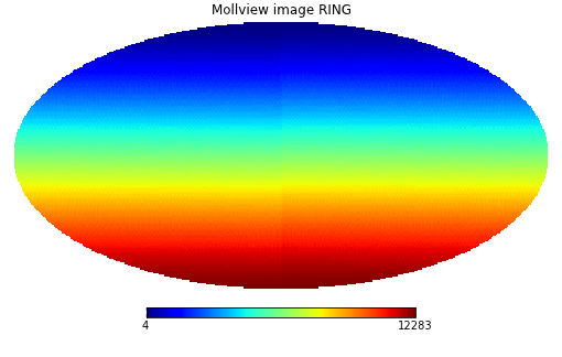
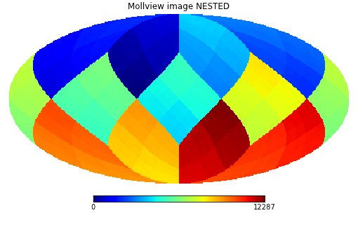
Healpix supports two different ordering schemes, RING or NESTED. By default, healpy maps are in RING ordering.

In order to work with NESTED ordering, all map related functions support the nest keyword, for example:

>>> hp.mollview(m, nest=True, title="Mollview image NESTED")

Reading and writing maps to file

Maps are read with the read_map() function:

>>> wmap_map_I = hp.read_map('../healpy/test/data/wmap_band_imap_r9_7yr_W_v4.fits')

By default, input maps are converted to RING ordering, if they are in NESTED ordering. You can otherwise specify nest=True to retrieve a map is NESTED ordering, or nest=None to keep the ordering unchanged.

By default, read_map() loads the first column, for reading other columns you can specify the field keyword.

write_map() writes a map to disk in FITS format, if the input map is a list of 3 maps, they are written to a single file as I,Q,U polarization components:

>>> hp.write_map("my_map.fits", wmap_map_I)

Visualization

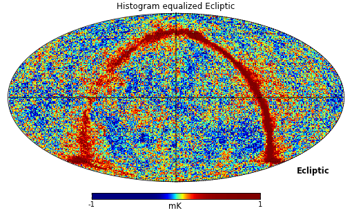
Mollweide projection with mollview() is the most common visualization tool for HEALPIX maps. It also supports coordinate transformation:

>>> hp.mollview(wmap_map_I, coord=['G','E'], title='Histogram equalized Ecliptic', unit='mK', norm='hist', min=-1,max=1, xsize=2000)
>>> hp.graticule()

coord does galactic to ecliptic coordinate transformation, norm=’hist’ sets a histogram equalized color scale and xsize increases the size of the image. graticule() adds meridians and parallels.

gnomview() instead provides gnomonic projection around a position specified by rot:

>>> hp.gnomview(wmap_map_I, rot=[0,0.3], title='GnomView', unit='mK', format='%.2g')

shows a projection of the galactic center, xsize and ysize change the dimension of the sky patch.

mollzoom() is a powerful tool for interactive inspection of a map, it provides a mollweide projection where you can click to set the center of the adjacent gnomview panel.

Masked map, partial maps

By convention, HEALPIX uses -1.6375e+30 to mark invalid or unseen pixels. This is stored in healpy as the constant UNSEEN().

All healpy functions automatically deal with maps with UNSEEN pixels, for example mollview() marks in grey that sections of a map.

There is an alternative way of dealing with UNSEEN pixel based on the numpy MaskedArray class, ma() loads a map as a masked array:

>>> mask = hp.read_map('../healpy/test/data/wmap_temperature_analysis_mask_r9_7yr_v4.fits').astype(np.bool)
>>> wmap_map_I_masked = hp.ma(wmap_map_I)
>>> wmap_map_I_masked.mask = np.logical_not(mask)

By convention the mask is 0 where the data are masked, while numpy defines data masked when the mask is True, so it is necessary to flip the mask.

>>> hp.mollview(wmap_map_I_masked.filled())

filling a masked array fills in the UNSEEN value and return a standard array that can be used by mollview. compressed() instead removes all the masked pixels and returns a standard array that can be used for examples by the matplotlib hist() function:

>>> import matplotlib.pyplot as plt
>>> plt.hist(wmap_map_I_masked.compressed(), bins = 1000)

Spherical harmonic transforms

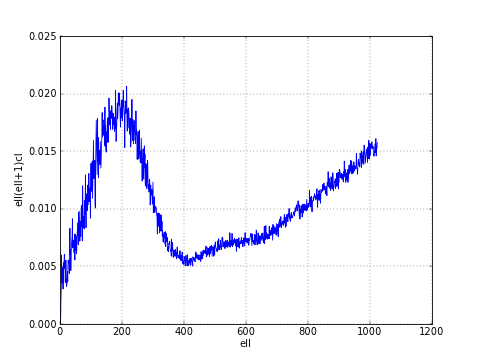
healpy provides bindings to the C++ HEALPIX library for performing spherical harmonic transforms. anafast() computes the angular power spectrum of a map:

>>> LMAX = 1024
>>> cl = hp.anafast(wmap_map_I_masked.filled(), lmax=LMAX)

the relative ell array is just:

>>> ell = np.arange(len(cl))

therefore we can plot a normalized CMB spectrum and write it to disk:

>>> plt.figure()
>>> plt.plot(ell, ell * (ell+1) * cl)
>>> plt.xlabel('ell'); plt.ylabel('ell(ell+1)cl'); plt.grid()
>>> hp.write_cl('cl.fits', cl)

Gaussian beam map smoothing is provided by smoothing():

>>> wmap_map_I_smoothed = hp.smoothing(wmap_map_I, fwhm=np.radians(1.))
>>> hp.mollview(wmap_map_I_smoothed, min=-1, max=1, title='Map smoothed 1 deg')